What is Fluorescence?
 Fluorescence is a form of luminescence (i.e. the emission of light not attributed to thermal radiation) that occurs over very short time scales – around 10-9 – 10-7s. The first fluorescent substance to be observed and recorded was quinine sulphate (a key ingredient in tonic water). In Figure 1 we can see fluorescence in action –the quinine sulphate molecules absorb, or are excited, by ultra-violet light (short wave radiation) from the laser pen and then emit blue light (longer wavelength radiation). Molecules that exhibit these properties are termed fluorophores.
The physical basis of fluorescence was first described and the term coined, by Sir George G. Stokes investigating the light emitting characteristics of fluorite in 1852. He identified that the wavelength (energy) of light emitted by a fluorophore was red shifted (i.e. of lower energy) than the light absorbed or that excited the molecules. However, the specific mechanisms and processes operating at the molecular/atomic level were not identified until the turn of the 20th Century. Alexander Jablonski was a key player in the development of fluorescence spectroscopy, and is best known for the Jablonski diagram (Figure 2); a succinct depiction of the complex processes involved in fluorescence.
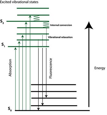 Figure 1 (left). The quinine sulphate molecules in tonic water emit blue light when exposed to high energy (UV) light.
Briefly, loosely held electrons of complex molecules can be excited to higher energy levels (i.e. S1) via absorption of a photon of light. Relaxation or non-radiative decay then occurs through collision or internal conversion. Finally emission of a photon (radiative decay) can occur from the lowest energy excited state to return the molecule to the ground state (stable electronic state – S0). An important property of fluorescence is that for a given molecule distinct absorption (excitation) and emission spectra are observed.
Figure 2 (right). Simplified Jablonski diagram. The electronic state is depicted Si. Rotational and vibrational energy levels are depicted as shorter lines.
Fluorescence spectroscopy: instrumentation
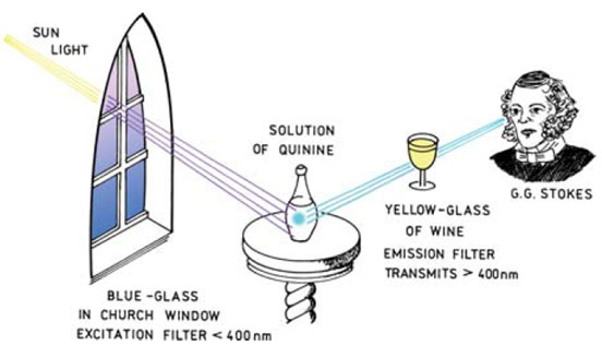
For fluorescence to be observed and quantified a light emitter and detector is required with some optical components for isolating specific wavelengths of light. Some of the earliest work on fluorescence carried out by Stokes involved the design of a simple fluorometer using an interesting set of components (Figure 3). The excitation light source was sunlight and a blue glass filter transmitted UV light, which was then absorbed by the quinine solution.
A yellow wine glass was used as a filter between the detector (Stokes) and the solution allowing the emitted (visible - 450 nm) light to be observed.
Figure 3 (below). An early experiment by Stokes highlights the components needed for a simple fluorometer.
This simple experiment highlights the principle components used in laboratory fluorometers today (Figure 4). Two types following similar design separated by the way in which the excitation and emission light is isolated from the wider spectrum: (i) filter based, or (ii) diffraction 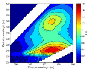 grating monochromator. The functional properties are similar: light from the excitation source is directed through a series consisting of lens and filters or a monochromator. When it reaches the sample the light is absorbed, and some of the molecules in the sample fluoresce. The fluorescent (emission) light passes through a second series of lens and filters/monochromator and reaches a detector (usually a photodiode). This photodiode is normally located 90° to the incident light beam to reduce the potential for spurious readings due to stray excitation light reaching the detector.
Over the past 30 years technological developments have meant rapid scanning across a range of excitation and emission wavelength pairs is possible using expensive, bench top fluorescence spectrophotometers (Figure 5). These instruments are able to provide 100’s of measurements in a matter of minutes. The output, an Excitation Emission Matrix (EMM; Figure 6) is a detailed map of the optical space occupied by a sample.
Figure 6 (left). An Excitation Emission Matrix of the treated effluent from a sewage treatment works
Why use fluorescence for monitoring water quality?
A significant proportion of chromophoric (light absorbing/coloured) organic matter is fluorescent when excited by light in the UV region. Distinct fluorescent peaks have been identified and related to certain ‘types’ of organic matter. For example, humic-like or CDOM fluorescence (Peak A and C on Figure 7) can be traced back to terrestrial production by vascular plants. Microbial or protein - like fluorescence (Peaks T and B; Figure 7) is largely related to in-stream production by algae and bacteria. These peaks show strong relationships with conventional water quality parameters such as Total Organic Carbon (correlated with humic-like fluorescence) and Biochemical Oxygen Demand (correlated with protein – like fluorescence).
Figure 7 (right). An Excitation Emission Matrix with the key peaks highlighted
Submersible fluorometers and real-time monitoring
Recently advances in LED technology have enabled the development of miniaturized UV fluorometers. There is now a range of commercially available, fully submersible low powered sensors for measuring organic matter fluorescence in real-time. The design 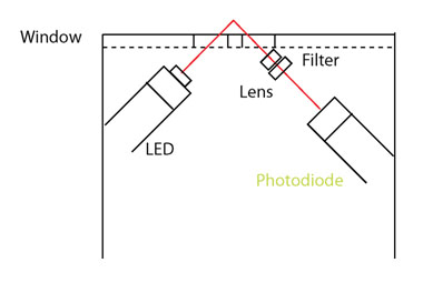 principle is identical to that of laboratory fluorometers except the light source is an LED rather than a lamp (Figure 8) and a filter is used rather than a monochromator. While this design only allows a single excitation-emission pair to be measured, fluorometers can be tuned to the wavelength pairs most suited to water quality monitoring. For example, humic-like fluorescence (i.e. CDOM: Ex 365 nm / Em 450nm) and protein like fluorescence (i.e. tryptophan-like Ex. 285 nm / Em 350nm) are widely used.
Figure 8 (right). Schematic representation of a submersible fluorometer
Challenges to in-situ monitoring
Fluorescence spectroscopy is a highly sensitive and selective optical technique that can now be used to quantify and characterise the composition of dissolved organic matter (DOM) in-situ. However, potential interferences need to be carefully considered before interpreting data. The following factors can quench (attenuate) and shift the signal wavelength:
- Temperature increases can reduce fluorescence intensity (quenching)
- Matrix interference from suspended particles can cause scattering/absorption (amplification or attenuation of the signal)
- Inner filtering or high concentration effect:
- Primary – absorption of the excitation beam
- Secondary– absorption of the emission photons
- Salinity quenching
- PH effects (very low or high pH can shift the peak wavelengths)
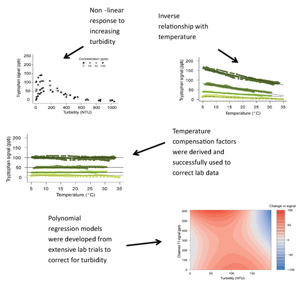
As part of a Knowledge Transfer Project RS Hydro have undertaking detailed research exploring potential temperature and turbidity effects on in-situ fluorescence measurements (see below). Robust temperature and turbidity correction procedures have been devised and rigorously tested and have been outlined in full in a peer reviewed article.